

This article briefly presents the most common approaches that are used to create a Digital Twin.
In the rapidly evolving world of digital twins and advanced control systems, the foundation of every successful project is a precise and reliable mathematical model. Systems theory allows us to uniformly describe the temporal behavior of highly diverse technical processes—from electrical and mechanical engineering to complex chemical plants.
But how do we derive these mathematical models? The process of capturing a system’s static and dynamic behavior essentially boils down to two fundamental approaches: theoretical modeling and experimental modeling. Understanding the differences, advantages, and synergies between these two approaches is critical for anyone developing Digital Twins.
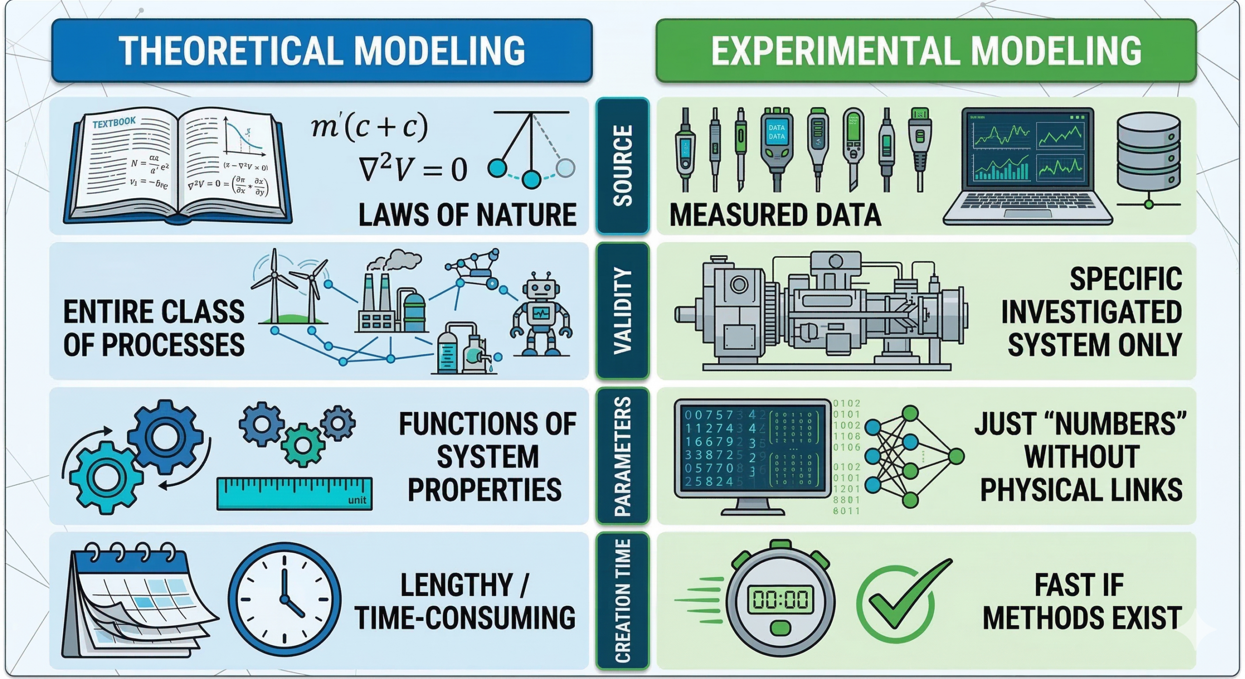
Theoretical Modeling: The “White-Box” Approach
Theoretical modeling (also known as theoretical analysis) builds a mathematical representation of a system strictly from the ground up, using fundamental laws of nature and physics. To build a theoretical model, engineers typically combine four distinct types of equations:
- Balance Equations: These account for the balance of mass, energy, and momentum within the system.
- Constitutive Equations: These describe reversible events, such as inductance in an electrical circuit or Newton’s second law in mechanics.
- Phenomenological Equations: These describe irreversible events, such as heat transfer or friction.
- Interconnection Equations: These define how different parts of the system interact, such as Kirchhoff’s node and mesh equations for electrical circuits or torque balances for mechanical drives.
By combining these equations, we obtain a set of ordinary or partial differential equations. Because the internal structure of the model is entirely known and based on physical reality, this is often referred to as a “White-Box” model.
Advantages and Limitations
The primary advantage is that it contains the direct functional dependencies between physical properties and parameters. It can be built for a non-existent system, making it invaluable during the design phase. On the other hand, analysis can become extraordinarily complex, often requiring simplifying assumptions that reduce accuracy.
Experimental Modeling: The “Black-Box” Approach
When physical laws are too complex or parameters are unknown, engineers turn to experimental modeling, widely known as System Identification. This approach involves observing actual input signals applied to the system and the resulting output signals.
By applying statistical methods to these measured signals, a model is formulated that mimics the behavior of the real process. Because the internal physics, or any mathematical structure, are often ignored, this is called a “Black-Box” model.
Advantages and Limitations
Experimental models usually describe the actual dynamic behavior of a specific system much more accurately than theoretical ones. This makes them the primary choice for tuning adaptive controllers. The main drawback is that parameters are meaningless “numbers”; there is no known functional relationship between the estimated parameters and the actual physical properties.
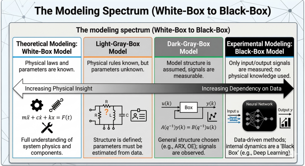
The Best of Both Worlds: Gray-Box Models
In modern digital twin applications, we rarely rely on a pure approach. Instead, we use “Gray Box” models. System analysis is an iterative procedure in which theoretical modeling establishes the basic structure (a “Light-Gray-Box”), and experimental identification estimates the unknown parameters.
There is also the “Dark-Gray-Box”, which identifies the parameters of a mathematical model that does not follow any physical rule and yet represents the behavior of the system being modeled. An example, assume a certain system has the behavior of a third-order linear system and only find the poles that describe it, without looking into physics.
In this category, hybrid approaches are included, e.g., modelling a UUV. An interesting part of modeling UUV behavior is to consider the effect of the displaced water around the body of the vehicle – Added Mass. Obviously, the fluid mechanics itself will not be encoded into the model explicitly, but we can encapsulate it using matrices (in fact, the full form is a tensor). This is where a neural network would be a good choice, while keeping the “traditional” part explicit: mass, inertia, etc.
Taxonomy of Model Types
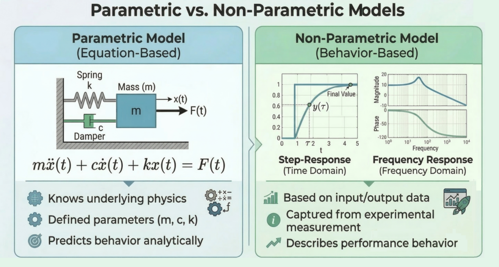
Whether derived theoretically or experimentally, models can also be classified into two primary categories:
| Model Type | Structure | Dimension | Example |
| Parametric | Explicitly defined | Finite | Differential equations, transfer functions. |
| Non-Parametric | Implicit/Tables | Infinite | Step responses, frequency response curves. |
Both types can be further subdivided into continuous-time models and discrete-time models (which are sampled in time and suitable for digital processing).
If you want to talk about these different approaches and their uses, send us a message. Either here, by email, or on LinkedIn!

Leave a Reply